Warming exacerbates global inequality in forest carbon and nitrogen cycles

Global synthesis of warming experiments in forests

We have compiled data from warming experiments (Supplementary Table 1) and additional open data sources to construct a comprehensive global dataset of warming experiments in forest ecosystems. We consulted the Manipulation Experiments Synthesis Initiative (MESI) database52 and performed a cross-search to identify eligible studies based on the following criteria (see Preferred Reporting Items for Systematic Reviews and Meta-Analyses, PRISMA flowchart as Supplementary Fig. 8): (1) warming experiments with control (ambient temperature) and treatment (elevated temperature) groups, including both field and incubation experiments; (2) measurements of variables associated with nitrogen and carbon cycles, such as BNF, N2O, NO3-, nitrogen/carbon content, NPP, soil respiration, and etc.; (3) studies published in peer-reviewed journals and indexed in authoritative databases such as Web of Science, Google Scholar, and Scopus. The systematic literature search focused on, but was not restricted to, these key terms: {(elevated temperature/increasing temperature/warming) AND {(forest/tree/seedling/shrub) AND {(nitrogen fixation/BNF/nitrogen use efficiency/NUE/denitrification/ammonia/NH3/nitrous oxide/N2O/nitrate/mineralization/nitrification/nitrogen) OR (net primary productivity/NPP/soil organic carbon/SOC/soil respiration/Rs/carbon)}.

From textual descriptions, tables, and figures, we extracted information about study sites, experimental design, and variable specifications. We used WebPlotDigitizer 4.4 (https://apps.automeris.io/wpd/) for data extraction from figures. In addition, we collected supplementary climate information, soil data, and climatic zone classifications for specific study sites from external open data sources when relevant information was missing. Historical and future climate data were obtained from the WorldClim database (https://worldclim.org/data/index.html#). Soil data were sourced from the Global Land Data Assimilation System (GLDAS) (https://ldas.gsfc.nasa.gov/gldas/soils). Climate zones were determined based on the Köppen-Geiger climate classification53.

We utilized multi-level meta-analyses organized into three tiers: (i) individual observations, (ii) climatic domain (such as boreal, temperate, (sub)tropical), and (iii) the global scale. An observation in the context of a forest warming experiment is a record of a variable of interest, including measurements from both the control and warming groups at a given time or for a given period of time.

To calculate the response ratio (effect size) for each individual observation, we utilized the natural logarithm of the response ratio (lnR) formula54, as shown below:

where \({x}_{{{{\rm{eT}}}}}\) and \({x}_{{{{\rm{aT}}}}}\) represent the means of parameters at elevated temperature and ambient temperature, respectively.

The weight assigned to each individual observation was determined according to the number of experimental replications, and the variance was calculated as the reciprocal of the weight using the following equations:

where \({n}_{{{{\rm{eT}}}}}\) and \({n}_{{{{\rm{aT}}}}}\) denote the number of replications at elevated temperature and ambient temperature levels, respectively.

We then calculated the weighted mean response ratios (RR) with 95% confidence intervals (CI) for tier ii and tier iii using a mixed effects model55, with ‘site’ included as a random factor to account for non-independence at the site level. The 95% CI defines the lower and upper bounds of the overall mean. An RR is considered statistically significant (P metafor package on the R platform (version 4.1.3)56. The results are presented as percentage changes in response ratios for clarity, using the following equation:

Carbon and nitrogen budgets in global forests

In this study, we estimated the global forest carbon and nitrogen budgets using DLEM30,31 and CHANS models32,33 (Supplementary Fig. 1). These estimates were generated at a spatial resolution of 0.5 degrees by 0.5 degrees. We adopted a multi-model simulation approach to establish robust global forest carbon and nitrogen budgets, aiming to minimize uncertainties. The gridded data generated by the DLEM model were systematically integrated into the CHANS model. This integration involved a comprehensive comparison and calibration process with the nationally-scaled data embedded within the CHANS model.

The DLEM model is a dynamic global vegetation model specifically designed to simulate daily variations in carbon, water, and nitrogen dynamics. It incorporates a wide range of factors, such as atmospheric chemistry, climate patterns, land-use changes, and disturbances31.

To calculate plant net primary productivity (NPPi) at the grid level i, the following equations were applied:

where GPPsun,i and GPPshade,i represent the gross primary productivity for the sunlit and shaded canopy, respectively; Gr,i represents the growth respiration of plants; Mr,i denotes the maintenance respiration; Asun,i and Ashade,i are the leaf-level assimilation rates of the sunlit and shaded canopy, respectively, calculated using the model proposed by Farquhar et al57.; LAIsun,i and LAIshade,i are the projected leaf area indices for the sunlit and shaded canopy, respectively; dayli denotes the duration of daylight in hours within a day.

The LAIsun is calculated using the following equation58:

where \(\Omega\) is a plant functional type (PFT) specific parameter to represent foliage clumping effect, LAI is the total leaf area index, \({{{{\rm{\theta }}}}}_{{{{\rm{ave}}}}}\) is daily average zenith angle.

The LAIshade is calculated using the following equation:

Maintenance respiration (Mr) of plants is influenced by surface air temperature and the carbon content present in various plant components, including leaves, sapwood, fine roots, and coarse roots. The calculation of Mr involves the aggregation of carbon pools across all plant parts as follows:

where Rsepcoef represents a respiration coefficient specific to each plant functional type; The temperature factor, denoted as f(T), is calculated as a function of the daily average air temperature; rmax represents the maximum respiration rate for different carbon pools; CVm corresponds to the carbon content of vegetation pool m.

The calculation of rmax is determined by the following equation:

\({{{\rm{where}}}}\) \({C}_{{{{\rm{seed}}}}}\) is PFT specific seed carbon. In order to simulate germination, vegetation carbon is assumed no less than \({C}_{{{{\rm{seed}}}}}\).

A \({Q}_{10}\) function is adopted to calculate temperature factor, \(f\left(T\right)\), as follows:

For aboveground biomass, such as leaf, sapwood, and reproduction pools, \(T\) is air temperature; for belowground pools such as coarse root and fine root, T is the average soil temperature of the upper 50 cm.

The calculation of the net biome productivity at time t (NBPt) is determined by the following equation:

where CVt, CSt, CLt, and CPt denote the carbon content of the vegetation pool, soil pool, litter pool, and product pool at time t, respectively; CVt-1, CSt-1, CLt-1, and CPt-1 represent the carbon content of these pools at time t-1, respectively.

The CHANS model is a nitrogen cycle model designed to simulate nitrogen flows within various interconnected subsystems at the interface of the natural and human environment32,33.

The calculation of the forest nitrogen budget is performed at the grid i level based on the mass balance principle using the following equations:

where \({{{{\rm{N}}}}}_{{{{\rm{input}}}},i}\) represents the total N input, consisting of BNF (NBNF,i), nitrogen deposition (Ndeposition,i), and synthetic fertilizer (Nfertilizer,i). Here, nitrogen fertilizer as a minor anthropogenic input is restricted to some managed forests, especially plantations and nitrogen-poor forests59,60,61 (Supplementary Fig. 9). \({{{{\rm{N}}}}}_{{{{\rm{input}}}},i}\) also equals to the sum of total nitrogen output, including reactive nitrogen (Nr,i), N2 emissions (N2,i), the quantity of nitrogen in both timber and non- timber forest products (Nproducts,i), and the N increment in living biomass, litterfall, and soil stock (Naccumulation,i); Nr,i includes gaseous NH3, N2O, and NOx emissions, as well as nitrate lossing to water bodies (NO3-); \({{{{\rm{NUE}}}}}_{i}\) denotes nitrogen use efficiency at grid i.

The loss factor (\({F}_{{{{\rm{loss}}}},i}\)) are defined as:

where Ncom,i could be any component of nitrogen loss; Nsurplus,i is the sum of reactive nitrogen and non-reactive N2.

Scenario design and model simulation

In this study, we formulated two sets of scenarios: (i) Baseline scenarios: These scenarios assume no climate change and encompass SSP1 (‘Sustainable society’), SSP2 (‘Middle road’), and SSP5 (‘Fossil-fueled society’). (ii) Warming scenarios: These scenarios focus solely on the impact of warming as the primary driver of climate change and include SSP1-2.6, SSP2-4.5, and SSP5-8.5, corresponding to ‘Sustainable society’, ‘Middle road’, and ‘Fossil-fueled society’, respectively. Future temperature projections under different socioeconomic pathways are Coupled Model Intercomparison Project Phase 6 (CMIP6) downscaled future climate projections from WorldClim database (https://worldclim.org/data/index.html#). Additionally, future forest areas were derived from the Global Change Analysis Model for future land use projections62.

Subsequently, we conducted model simulation under various scenarios. The effects of warming on forest carbon and nitrogen variables were integrated into the forest products based on climatic domain and temperature optima of vegetation productivity under future warming scenario within grid i using the following equations:

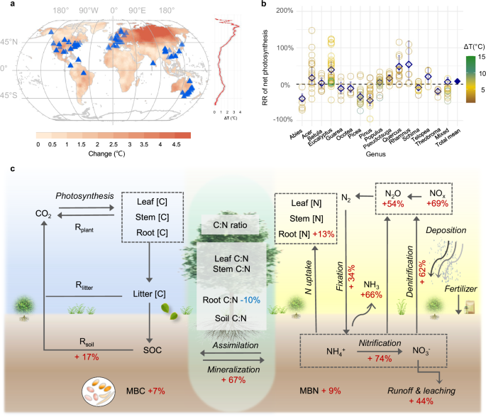
where \({{{{\rm{N}}}}}_{{{{\rm{products}}}},i}^{{{{\rm{eT}}}}}\) and \({{{{\rm{N}}}}}_{{{{\rm{products}}}},i}^{{{{\rm{base}}}}}\) represent the nitrogen in the forest products under the warming scenario and baseline scenario, respectively; \({{{{\rm{RR}}}}\%}_{{{{\rm{NPP}}}},i}\) and \({{{{\rm{RR}}}}\%}_{{{{\rm{stem}}}}[{{{\rm{N}}}}],i}\) denote the response ratios of NPP and stem nitrogen content to warming. Here net photosynthesis is used as a proxy for NPP in the meta-analysis. When the temperature optima of the productivity are exceeded, the negative response is dominant in the forest or the positive response is dominant (Supplementary Fig. 10). The temperature optima of vegetation productivity for different climatic domains were obtained from a previous global synthesis21.

The total nitrogen input under warming (\({{{{\rm{N}}}}}_{{{{\rm{input}}}}}^{{{{\rm{eT}}}}}\)) is obtained by summing up all the nitrogen input components within grid i as follows:

where the BNF under the warming scenario (\({{{{\rm{N}}}}}_{{{{\rm{BNF}}}},i}^{{{{\rm{eT}}}}}\)) is attained by integrating the effects of warming and the optimal temperature8 on the base BNF rates; nitrogen deposition under the warming scenario (\({{{{\rm{N}}}}}_{{{{\rm{deposition}}}},i}^{{{{\rm{eT}}}}}\)) is obtained by integrating the effects of warming on baseline nitrogen deposition as a function of summed NH3 and NOx emissions; fertilizer application is assumed to maintain a uniform rate per unit of forest area fertilized.

As for the calculation of nitrogen loss, the effects of warming were incorporated to the component of nitrogen loss within grid i as follows:

where \({{{{\rm{N}}}}}_{{{{\rm{loss}}}},i}^{{{{\rm{eT}}}}}\) and \({{{{\rm{N}}}}}_{{{{\rm{loss}}}},i}^{{{{\rm{base}}}}}\) represent the nitrogen loss under the warming and baseline scenarios, respectively; \({{{{\rm{RR}}}}\%}_{{{{\rm{Ncom}}}},i}\) denotes the response ratio of any nitrogen loss component to warming. Since NH3 and NOx emissions from forests are minimal and metadata are insufficient, we use terrestrial mean response ratios as proxies.

The biome C: N ratio (CNbio) is calculated within grid i using the following equation:

It is assumed that CNbio under warming remains similar to that in baseline, according to the results of the meta-analysis. Here, Nproducts,i and Naccumulation,i are calibrated to account for the effects of warming in the warming scenarios. Consequently, NBP is calculated under the warming scenarios using the formula mentioned above.

Impact assessment

The economic impact analysis of warming (\({I}_{{{{\rm{eT}}}}}\)) as the sole driver of climate change is carried out at the grid level within global forests. This analysis takes into account the potential effects on various aspects, including ecosystem (\({I}_{{{{\rm{eco}}}}}\)), climate change (\({I}_{{{{\rm{climate}}}}}\)), and forest production (\({I}_{{{{\rm{pro}}}}}\)) within grid i, as outlined below:

The impact on the ecosystem is measured by calculating the changes in damage costs resulting from Nr effects within grid i, as expressed in the following equation63,64:

where \(\Delta {{{{\rm{N}}}}}_{r,i}\) represents the change in Nr under warming scenario relative to the baseline, encompassing NH3, N2O, NOx, and NO3- losses at grid i; \({d}_{{{{\rm{eco}}}},{{{\rm{EU}}}}}\) represents for the estimated ecosystem damage cost of Nr emission in the European Union (EU) based on the European N Assessment; \({{{{\rm{WTP}}}}}_{j}\) and \({{{{\rm{WTP}}}}}_{{{{\rm{EU}}}}}\) denote the values of the willingness to pay for ecosystem service in the country/ area j and the EU, respectively; \({{{{\rm{PPP}}}}}_{j}\) and \({{{{\rm{PPP}}}}}_{{{{\rm{EU}}}}}\) denote the purchasing power parity of the country/ area j and the EU. To account for data limitations, we extend the ecosystem damage cost of Nr emissions in the EU to other countries by applying adjustments for comparable ecosystem benefits worldwide using willingness to pay and purchasing power parity adjustments.

The assessment of climate impact is conducted by taking into account the influence of carbon sequestration and Nr losses on climate change within grid i, as described below65:

where the change in C sequestration under warming is estimated by multiplying change of carbon sequestration (\(\Delta {{{{\rm{C}}}}}_{i}\)) and the carbon price (\({p}_{{{{\rm{C}}}},{i}}\)); we use the national carbon prices for calculation66, and the missing values for some countries are supplemented with means of the income groups; the influence of Nr losses on climate change is estimated by multiplying change of Nr losses (\(\Delta {{{{\rm{N}}}}}_{r,i}\)) and climate damage cost of Nr (\({d}_{{{{\rm{climate}}}},i}\)). The effects of Nr on climate change can be positive or negative, i.e., N2O contributes to climate warming as a potent greenhouse gas, while NOx and NH3 exert climate cooling give that they are precursors of aerosol reflecting long-wave solar radiation.

The monetary evaluation of forest production is performed by subtracting the production costs from the income generated by forest products. Production costs here primarily refer to fertilizers, while other costs such as infrastructure (i.e., road construction) and logging operations are not considered in this study. The equation used is as follows:

where \(\Delta {{{{\rm{N}}}}}_{{{{\rm{pro}}}},i}\) denotes the changes in forest products under warming; the price of forest products (\({p}_{{{{\rm{pro}}}},{i}}\)) is estimated by dividing the value of forest products traded by the quantity based on the FAO database (https://www.fao.org/faostat/en/#data/FAO);\(\,\Delta {{{{\rm{N}}}}}_{{{{\rm{fertilizer}}}},i}\) denotes the changes in N fertilizer under warming; the N fertilizer price (\({p}_{{{{\rm{fertilizer}}}},{i}}\)) is estimated by dividing the value of fertilizers traded by the quantity based on the UN Comtrade Database (https://comtrade.un.org/). For countries with missing price data, we substitute the global average value.

Uncertainty analysis

To comprehensively assess model output uncertainties, we conducted an uncertainty analysis using Monte Carlo simulations with the CHANS model. We performed 1000 iterations to generate projection ensembles and calculate both the mean and variability of carbon and nitrogen budgets. Coefficients of variation (CV) were used to gauge the relative levels of uncertainty in carbon and nitrogen budgets data and the effects of warming on carbon and nitrogen dynamic (Supplementary Table 2).

Reporting summary

Further information on research design is available in the Nature Portfolio Reporting Summary linked to this article.