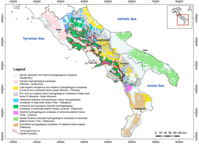
The territory of southern Italy is characterized by a high heterogeneity and complexity of geological-structural and hydrogeological features. The principal hydrogeological features of the southern Italy can be summarized in nine hydrogeological domains30 which, in decreasing order of relevance for what regards the mean annual specific groundwater yield (Fig. 1), can be identified as: (a) Mesozoic carbonate series that, depending on hydrogeological features, can be arranged in four subgroups: calcareous-siliceous, limestone, dolomitic, carbonate and Apulian foreland carbonate aquifers; (b) Plio-Quaternary alluvial and epiclastic deposits; (c) volcanic rocks and soils of Plio-Quaternary eruptive centres; (d) Paleozoic crystalline-metamorphic rocks of the Calabrian arch; (e) Cretaceous-Cenozoic basin series, which mainly constitute the minor mountainous or hilly reliefs of the southern Apennines.
Hydrogeological map of the continental southern Italy showing the nine principal hydrogeological domains30. Hydrogeological boundaries of karst aquifers are also shown. The map was created using QGIS software (v. 3.34; https://qgis.org/).
In such interregional framework, the study area includes the entire portion of the western sector of the southern Apennines (about 19,339 km2), where Mesozoic carbonate series, forming high mountain ranges, outcrop and constitute very extended karst aquifers characterized by high permeability due to fracturing and karst phenomena (Fig. 1). These karst aquifers are characterized by limestone, limestone-dolomite and dolomite rocks, ranging in age from Triassic to Upper Cretaceous, derived from the tectonic disintegration of the carbonate platform that occurred during the Miocene tectonic phases31,32. In southern Italy, karst aquifers cover the 45%33 of the territory hosting the major groundwater resources which supply drinkable, industrial and thermos-mineral uses as well as contributing to the equilibrium of river ecosystems. This is favoured by the peculiar geological-structural, hydrogeological, geomorphological and climatological settings of the region which determine the occurrence of several high-permeability karst aquifers, with a high mean annual groundwater recharge and circulation rates.
Given their importance, many studies have been carried out on the karst aquifers of southern Italy regarding: (i) hydrogeological characterization and the mapping of groundwater resources30,34,35; (ii) groundwater recharge estimation at the different spatio-temporal scales and by terrestrial and satellite datasets33,36,37,38; (iii) groundwater vulnerability to pollution39,40, microbial contamination and environmental impact of cattle grazing on karst groundwater41. The Plio-Quaternary deposits, which include deposits of alluvial plains, coastal plains and intermontane basins, outcropping for about 24,500 km2, which are directly recharged by effective or secondary infiltration from watercourses, thus receiving lateral groundwater inflow from the adjoining karst aquifer systems.
The lateral confinement of karst aquifers by low-permeability terrains constrains the groundwater circulation toward huge basal springs which are often characterized by high flows up to a few m3/s34,42,43, and predisposed to the effective tapping. Therefore, karst aquifers represent the main source of groundwater for southern Italy, providing an estimated average annual water volume of approximately 4100 × 106 m3 · year–1 with a mean specific annual groundwater yield up to 0.035 m3 · s–1 · km–2.30
The principal regional aqueducts are supplied by the tapping by gravity of the main basal springs of karst aquifers, in most cases not provided by pumping systems, therefore the availability of groundwater resources of these aquifers correspond to their natural recharge.
Climate models
To investigate the future climate projections and the related impacts on groundwater recharge processes over the study area (Fig. 2), annual precipitation and mean air temperature data from the EURO-CORDEX simulations25 were achieved from the nodes of the earth system grid federation (ESGF).
(a) Map of the modelled study area showing the distributions of air temperature and rain gauge stations (OBS) which functioned, even discontinuously, in the calibration period (1950–1996); (b) EUR-11 RCMs grid. Karst aquifers (green colour) of the southern Apennines area also shown in both maps. The maps were created using QGIS software (v. 3.34; https://qgis.org/).
Specifically, 15 different combinations of GCMs/RCMs were selected (Table 2). RCMs selected belong to the subset EUR-11 with a resolution of 0.11° (about 12.5 km) (Fig. 2b). Accordingly, data available for the “historical experiment” period (from 1950/1970 to 2005) and scenarios (from 2006 to 2099/2100) were analysed in this research. As already mentioned, RCP4.5 and RCP8.5 scenarios were selected, being the RCP8.5 the most severe (“business as usual”), while the RCP4.5 is representative of intermediate conditions.
According to other studies developed with a general purpose and in different geographical frameworks44,45,46,47,48, the RCP 8.5 is commonly used because representing the most extreme conditions, even if being the least likely49. As a result, an ensemble of 15 RCMS (E15; Table 2) was reconstructed, re-projected in WGS84-UTM 33N and analysed.
Observed precipitation and air temperature time series (1950–1996)
In the southern Italy, as well as for the rest of the national territory, a hydrological monitoring has been carried out since 1921 by means of a dense monitoring network, managed by the SIMN governmental agency and consisting in a numerous series of rain gauges and air temperature stations.
In the study area, the management of the monitoring network was in charge of the Department of Naples of the SIMN, which operated in a territory covering a large part of southern Italy, comprising the study area (Fig. 2a). The meteorological monitoring network was provided initially by mechanical rain gauges, based on the accumulation of the daily rainfall, and air temperature stations.
Starting from 1921, the number of rain gauges and air temperature stations was progressively increased and improved technologically until reaching a total of 423 stations in 1999. The recorded data, after a process of validation, were published in the annals by the aggregation of data from daily, to monthly and annual temporal scales.
The meteorological network undergone different changes during the period 1921–1999 due to the progressive increase of the number of stations as well as their discontinuous activity, because of temporary malfunctioning or abandonment during the World War II as well their relocation. These continuous changes of the monitoring network resulted in time series discontinuous in space and time.
Notwithstanding these issues, the huge database of historical meteorological data was considered very relevant for the comparison with RCMs data of the “historical experiments” periods (from 1950/1970 to 2005) and innovative for the regional scale of analysis, instead of the more common site-specific one, as well as challenging for its discontinuous functioning in space and time. Therefore, annual precipitation and mean annual air temperature were extracted by the annals of the SIMN, made of public access by a dedicated project of Italian Institute for Environmental Protection and Research (ISPRA), and filed in a database covering the period 1950–1996. In detail, annual precipitation and mean annual air temperature data were extracted for each of the available monitoring stations, which were considered as observation points (OBS). The OBS data were used for a statistical comparison to the E15 ones at the regional scale, by considering both types of data comprised in each of the grid cells of the RCMs (~ 12 km) (Fig. 2a and b). A total of 143 RCMs grid cells were recognized comprising rain gauge stations, while 96 air temperature stations.
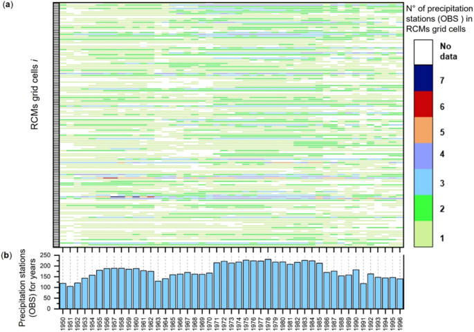
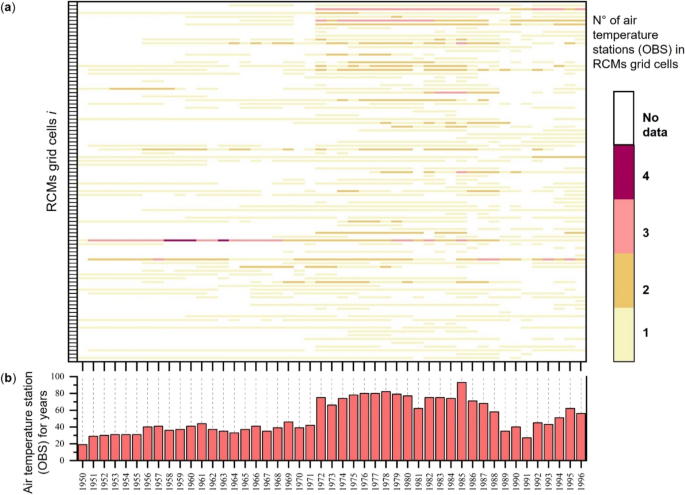
In order to represent the spatial and temporal variability of rain gauge and air temperature stations comprised in the cells of the RCMs, a representation in the form of heat map was carried out respectively (Figs. 3 and 4).
By the analysis of spatial and temporal distribution of rain gauges in the grid cells of RCMs (Fig. 2b) a minimum number of 100 functioning rain gauges in 1951 and 1991 and a maximum of 225 in 1978 was recognized (Fig. 3). The coverage of each grid cell of RCMs with at the least one rain gauge, up to six, prevails on cells with no rain gauges.
Regarding the spatial and temporal distribution of air temperature stations in the grid cells of RCMs (Fig. 4), the minimum number of 20 occurred in 1950 and a maximum of 96 in 1985. The coverage of each cell with no air temperature stations prevails on those comprising at least one. The latter were recognized encompassing up to four air temperature stations for each grid cell. The lower spatial density of air temperature stations in comparison to that of rain gauges is due to the lower spatial variability of the air temperature which is mostly controlled by the altitude only.
RCMs processing: bias assessment and correction
All the RCMS data (precipitation and air temperature) were pre-processed with the climate data operators (CDO) software50, which is a collection of operators and tools for standard processing of climate and forecast model data in NetCDF format. The operators include arithmetic functions, data selection and subsampling tools and spatial interpolation.
For each model, the pre-processing has involved the aggregation of the NetCDF datasets and the conversion of the units of precipitation (from kg·m2·s–1 to mm·h–1) and air temperature (from K to °C). Furthermore, the precipitation and air temperature data from RCMs (based on a 360-day calendar) were adjusted by linear interpolation to align with the standard Gregorian calendar. Therefore, a subset of data related to the area of the southern Apennines was extracted (Fig. 2b).
RCMs data need the application of a bias correction technique, aimed to the removal of systematic errors. Which is performed considering a period in which observed (OBS) and modelled time series are available and overlapped9.
Different methodologies for the bias correction have been developed and are available in literature28, depending on the choice of the method on both the type of the observed data available and the goal of the study9.
Bias-correction methods require daily or monthly time-series over a period of at least 30 years51. The purpose of this stage of data processing was to assess the differences existing between the RCMS “historical experiments” datasets and the measured data (OBS) in the considered period (1950–1996). Data elaboration was performed with the high-level functions NetCDF Library Package of MATLAB® (R2021b) applicable for reading and processing climate variables from NetCDF data files. Specifically, a method based on inferential statistical studies of the bias was adopted. In order to allow the comparison between the E15 and OBS data, two pairs of datasets were created, based on the recognition of grid cells of the RCM model within which OBS precipitation (OBSP) and OBS air temperature (OBST) resulted available (Fig. 5a and b).
(a) rain gauges and (b) air temperature stations which functioned in the calibration period 1950–1996. The RCMs grid cells which comprised at least one monitoring station are also represented. The maps were created using QGIS software (v. 3.34; https://qgis.org/).
For each year, OBSP and OBST given at each grid cell were compared with the E15 precipitation (E15P) and air temperature (E15T) data related to the same grid cell (Fig. 5a and b). In the case of multiple stations occurring in the same grid cell, mean values of OBSP and OBST were calculated and compared with the corresponding E15P and E15T data. The bias analysis between E15P and OBSP and between E15T and OBST was carried for every grid cell at the annual scale by the equation Eq. (1):
$${Bias}_{P,T,t}\left(j\right)=\frac{({Model}_{P,T,t}\left(j\right)-{OBS}_{P,T,t}\left(j\right))}{{OBS}_{P,T,t}(j)} ,$$
(1)
where \({Model}_{P,T,t}(j)\) is the value of E15P or E15T and \({OBS}_{P,T,t}(j)\) is the observed value of precipitation or air temperature for the year t (t = 1950, 1951…1996) in the jth grid cell.
Then, the mean value of the bias over the generic tyear (\(\overline{{Bias }_{P,T,t}}\)) and the whole area, was calculated by Eq. (2):
$$\overline{{Bias }_{P,T,t}}=\frac{{\sum }_{j=1}^{n}{Bias}_{P,T}(j)}{{\sum }_{j=1}^{n}j},$$
(2)
In which n indicates the number of grid cells considered. Finally, the bias-corrected annual value of the E15 (\({Model}_{P,T,t}^{*}(j)\)) is then evaluated by Eq. (3):
$${Model}_{P,T,t}^{*}\left(j\right)={Model}_{P,T,t}\left(j\right) \times \left(1-\overline{{Bias }_{P,T}} \right).$$
(3)
Hydro-climatological scenarios
The evaluation of the long-term effects of climate change on hydrological variables controlling groundwater recharge of karst aquifers was carried out considering the E15 bias-corrected values of precipitation and air temperature. Among the different hydrogeological domains, the spatial analyses were carried out on the areas of karst aquifers (Fig. 2a and b), which were considered the most relevant for the assessment of the impact of climate change on groundwater recharge due to their hydrogeological relevance. Accordingly, all the E15 grid cells intersecting the boundaries of the karst aquifers were extracted from the whole E15 dataset, and time series of mean annual precipitation and air temperature were created for reconstructing a complete time series including both the “historical experiment” period (1950–2005) and scenarios (2006–2100) under both the RCP4.5 and RCP8.5 pathways.
The evaluation of the climate change impact on groundwater recharge was assessed through the application of the hydrological budget equation Eq. (4):
$${P}_{tj}={ETR}_{tj}+{Ie}_{tj}+{R}_{tj},$$
(4)
where \({P}_{tj}\) is the precipitation, \({ETR}_{tj}\) is the actual evapotranspiration, \({Ie}_{tj}\) is the effective infiltration or groundwater recharge and \({R}_{tj}\) is the runoff, respectively related to the tyear and jcell.
The ETR was estimated by the Turc empirical formula52,53 Eq. (5):
$${ETR}_{t,j}= \frac{{P}_{t,j}}{\sqrt{0.9+{\left(\frac{{P}_{t,j}}{300+25*{T}_{t,j}+0.05*{T}_{t,j}^{3}}\right)}^{2}}},$$
(5)
where \({P}_{t,j}\) is the total annual precipitation (mm) and \({T}_{t,j}\) is the mean annual air temperature (°C), both for the jcell.
The Turc formula is commonly considered applicable to all different climates, either humid, arid, hot or cold because it was reconstructed by the application of the water balance equation to precipitation and runoff data of 254 drainage basins of Europe, Africa, America and the East Indies. In addition, the applicability of the Turc formula to the climate conditions of southern Italy has already been positively tested through a comparison with the results obtained by the other empirical formulas of Coutagne54 and Thorntwaite55 as well as with MODIS satellite estimations33.
Since the Turc formula depends on the annual precipitation (P) and mean annual air temperature (T), it intrinsically incorporates the spatial heterogeneity of these two hydrological variables. Therefore, the formula was applied to all grid cells for which P and T data were reconstructed by the E15 for each year of the time series.
From Eqs. (4) and (5), the effective precipitation \({Pe}_{t,j}\) of the tyear and jcell was considered as a proxy hydrological parameter describing the amount of precipitation potentially available groundwater recharge process and, therefore, useful for assessing the related effects of climate change scenarios Eq. (6):
$${Pe}_{tj}={P}_{tj}-{ETR}_{tj}=+{Ie}_{tj}+{R}_{tj}.$$
(6)
The reconstruction of Pe time series until 2100 is considered a fundamental step to assess the groundwater recharge by the application of empirical approach based on the multiplication by a factor known as Annual Groundwater Recharge Coefficient – AGRC37, which is suitable at the annual and regional scales.
Finally, to investigate the variation of Pe relatively to the “historical experiment” period (1950–2005), the mean annual effective precipitation index (MAEPI)56 was calculated for each year of the time series and the whole area, as follows Eq. (7):
$${MAEPI}_{t}=\frac{{Pe}_{t}- {Pe Hist}_{t}}{{Pe Hist}_{t}},$$
(7)
where MAEPIt is the Mean Annual Effective Precipitation Index for the tyear (%), Pet is the Effective Precipitation for the tyear and PeHistt is the Mean Annual Effective Precipitation of the whole E15 time series, corresponding to the “historical experiment” period (1950–2005), and the whole area.


